Regret Analysis of FTRL and OMD Algorithms

Introduction

In this note, we’ll explore the regret analysis of both the Follow-The-Regularized-Leader (FTRL) algorithm and the Online Mirror Descent (OMD) algorithm. We’ll highlight their similarities and differences, and demonstrate how, under certain conditions, they are essentially equivalent. This analysis includes detailed derivations and mathematical expressions.

Follow-The-Regularized-Leader (FTRL)

Problem Setup

Consider an online convex optimization problem over \( T \) rounds. At each round \( t \):

1. Decision Making: The learner selects \( \mathbf{x}_t \in \mathcal{X} \subseteq \mathbb{R}^n \).
2. Loss Revealing: An adversary reveals a convex loss function \( f_t : \mathcal{X} \rightarrow \mathbb{R} \).
3. Loss Incurred: The learner incurs loss \( f_t(\mathbf{x}_t) \).

Goal: Minimize the cumulative regret:

FTRL Algorithm

At each round \( t \), the FTRL algorithm updates the decision by solving:

where:

• \( \eta > 0 \) is the learning rate.
• \( R : \mathcal{X} \rightarrow \mathbb{R} \) is a strongly convex regularization function.

Regret Analysis

Assumptions

1. Convexity: Each loss function \( f_t \) is convex.
2. Lipschitz Continuity: The subgradients are bounded: \( \| \nabla f_t(\mathbf{x}) \|_* \leq G \) for all \( \mathbf{x} \in \mathcal{X} \).
3. Strong Convexity: The regularizer \( R \) is \( \lambda \)-strongly convex with respect to a norm \( \| \cdot \| \).

Key Steps

1. One-Step Regret Bound

   Using the convexity of \( f_t \):

   \[ f_t(\mathbf{x}_t) - f_t(\mathbf{x}^*) \leq \langle \nabla f_t(\mathbf{x}_t), \mathbf{x}_t - \mathbf{x}^* \rangle, \]

   where \( \mathbf{x}^* = \arg\min_{\mathbf{x} \in \mathcal{X}} \sum_{t=1}^T f_t(\mathbf{x}) \).

2. Regret Decomposition

   Summing over \( t \):

   \[ \text{Regret}_T \leq \sum_{t=1}^T \langle \nabla f_t(\mathbf{x}_t), \mathbf{x}_t - \mathbf{x}^* \rangle. \]

3. Bounding the Inner Product

   Using the properties of the regularizer and the FTRL updates, we can relate the sum to the Bregman divergence \( D_R \):

   \[ \sum_{t=1}^T \langle \nabla f_t(\mathbf{x}_t), \mathbf{x}_t - \mathbf{x}^* \rangle \leq \frac{R(\mathbf{x}^*) - R(\mathbf{x}_1)}{\eta}. \]

   Bregman Divergence Definition:

   \[ D_R(\mathbf{x}, \mathbf{y}) = R(\mathbf{x}) - R(\mathbf{y}) - \langle \nabla R(\mathbf{y}), \mathbf{x} - \mathbf{y} \rangle. \]

4. Regret Bound

   Therefore, the total regret is bounded by:

   \[ \text{Regret}_T \leq \frac{R(\mathbf{x}^*) - R(\mathbf{x}_1)}{\eta}. \]

   By choosing \( \eta \) appropriately (e.g., \( \eta = \sqrt{\dfrac{2 [R(\mathbf{x}^*) - R(\mathbf{x}_1)]}{G^2 T}} \)), we can achieve a regret bound of:

   \[ \text{Regret}_T \leq G \sqrt{2 [R(\mathbf{x}^*) - R(\mathbf{x}_1)] T}. \]

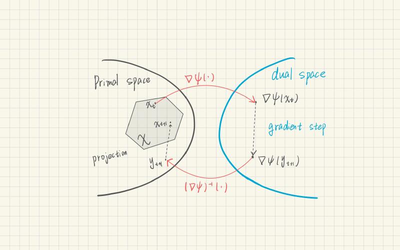
Online Mirror Descent (OMD)

Algorithm Steps

1. Initialization: Choose an initial point \( \mathbf{x}_1 \in \mathcal{X} \).

2. For each round \( t = 1, \dots, T \):

   a. Compute Subgradient:

   \[ \mathbf{g}_t = \nabla f_t(\mathbf{x}_t). \]

   b. Dual Space Update:

   \[ \mathbf{z}_{t+1} = \mathbf{z}_t - \eta \mathbf{g}_t, \]

   where \( \mathbf{z}_t = \nabla \psi(\mathbf{x}_t) \).

   c. Primal Space Update:

   \[ \mathbf{x}_{t+1} = \nabla \psi^*(\mathbf{z}_{t+1}), \]

   with \( \psi^* \) being the convex conjugate of \( \psi \).

Regret Analysis

Assumptions

1. Convexity: Each \( f_t \) is convex.
2. Lipschitz Continuity: Subgradients are bounded: \( \| \mathbf{g}_t \|_* \leq G \).
3. Strong Convexity: The mirror map \( \psi \) is \( \lambda \)-strongly convex.

Key Steps

1. Regret Decomposition

   The regret can be bounded by:

   \[ \text{Regret}_T \leq \sum_{t=1}^T \langle \mathbf{g}_t, \mathbf{x}_t - \mathbf{x}^* \rangle. \]

2. Using Mirror Descent Updates

   Utilizing the properties of the Bregman divergence \( D_\psi \) and the mirror descent updates:

   \[ \sum_{t=1}^T \langle \mathbf{g}_t, \mathbf{x}_t - \mathbf{x}^* \rangle = \frac{1}{\eta} \left[ D_\psi(\mathbf{x}^*, \mathbf{x}_1) - D_\psi(\mathbf{x}^*, \mathbf{x}_{T+1}) + \sum_{t=1}^T D_\psi(\mathbf{x}_{t+1}, \mathbf{x}_t) \right]. \]

3. Bounding the Bregman Divergences

   Since \( D_\psi(\mathbf{x}^*, \mathbf{x}_{T+1}) \geq 0 \) and \( D_\psi(\mathbf{x}_{t+1}, \mathbf{x}_t) \leq \dfrac{\eta^2 G^2}{2 \lambda} \), we have:

   \[ \text{Regret}_T \leq \frac{D_\psi(\mathbf{x}^*, \mathbf{x}_1)}{\eta} + \frac{\eta G^2 T}{2 \lambda}. \]

4. Optimizing the Learning Rate

   Choosing:

   \[ \eta = \sqrt{\dfrac{2 \lambda D_\psi(\mathbf{x}^*, \mathbf{x}_1)}{G^2 T}}, \]

   yields the regret bound:

   \[ \text{Regret}_T \leq G \sqrt{\dfrac{2 D_\psi(\mathbf{x}^*, \mathbf{x}_1) T}{\lambda}}. \]

Equivalence of FTRL and OMD

Under certain conditions, FTRL and OMD are equivalent algorithms.

Conditions for Equivalence

• Matching Regularizers and Mirror Maps: If the regularizer \( R \) in FTRL is identical to the mirror map \( \psi \) in OMD.
• Unconstrained Domain: When the feasible set \( \mathcal{X} \) is the entire space \( \mathbb{R}^n \).

Demonstration of Equivalence

1. FTRL Update in Terms of Gradients

   The FTRL update can be expressed as:

   \[ \mathbf{x}_t = \arg\min_{\mathbf{x} \in \mathcal{X}} \left\{ \left\langle \eta \sum_{s=1}^{t-1} \mathbf{g}_s, \mathbf{x} \right\rangle + R(\mathbf{x}) \right\}. \]

2. Relation to Dual Variables in OMD

   In OMD, the dual variable \( \mathbf{z}_t \) is:

   \[ \mathbf{z}_t = \nabla \psi(\mathbf{x}_t) = \mathbf{z}_1 - \eta \sum_{s=1}^{t-1} \mathbf{g}_s. \]

3. Primal Update via Convex Conjugate

   The FTRL update becomes:

   \[ \mathbf{x}_t = \nabla R^*\left( -\eta \sum_{s=1}^{t-1} \mathbf{g}_s \right), \]

   which matches the OMD update when \( R = \psi \):

   \[ \mathbf{x}_t = \nabla \psi^*\left( \nabla \psi(\mathbf{x}_1) - \eta \sum_{s=1}^{t-1} \mathbf{g}_s \right). \]

Conclusion

By aligning the regularization function in FTRL with the mirror map in OMD and considering the unconstrained domain, the updates of both algorithms coincide. This demonstrates that FTRL and OMD are essentially equivalent under these conditions, offering different perspectives on the same optimization process.